Microbiome
Introductory project from SNU
Microbiome Data Analysis Tutorial
This is a microbiome data analysis tutorial for the lab that I made.
Library
The necessary libraries are following.
# BiocManager::install("phyloseq")
library(phyloseq)
library(dplyr)
library(data.table)
library(stringr)
Load .biome data
There are four forms of phyloseq class data.
- otu_table : OTU count data
- sample_data : Sample data
- tax_table : Taxonomy data
- phy_tree : Phylogentic Tree data
Generate Phylogenetic Tree
Using the information of Denovo, we can generate the phylogenetic tree.
- adegenet : A package that includes the function, fasta2DNAbin, loading
.fastadata. - ape : This package can generate
Phylogentic Tree
# install.packages("ape")
# install.packages("adegenet")
library(adegenet)
library(ape)
Then you can load fasta data.
dna <-fasta2DNAbin("F:/work/Microbiome_EDC/HN00117382_Reports/otus_rep.fasta")
class(dna)
dna
There are several options to create Tree. You can check from ?dist.dna(). Importantly, if there is missing value in the distance matrix, you can only use njs() function. Otherwise, nj() can be applicable.
It takes longer than your thonght, so please save the results.
D <- dist.dna(dna, model = "raw")
length(D)
tre <- nj(D)

D <- dist.dna(dna, model = "TN93")
length(D)
tre <- njs(D)

save(tre, file = "F:/work/Microbiome_EDC/RData/TN93_tre.RData")
You can load your results from the following code.
load("F:/work/Microbiome_EDC/RData/TN93_tre.RData")
You can assign the loaded tree to the phyloseq form data.
tre$tip.label <- sapply(strsplit(tre$tip.label, "\t"), function(x)x[1])
phy_tree(data) <- tre
data
Lastly, if you want to separate your phyloseq data, do the following.
otu <- otu_table(data)
sample_dat <- sample_data(data)
tax <- tax_table(data)
phy_tre <- phy_tree(data)
Managing phyloseq data
You can check the ranking level of taxonomy by rank_names() function. ```{r, results = ‘markup’} rank_names(data) tax_table(data) %>% colnames
And add the label of the ranking.
```{r, results='markup'}
colnames(tax_table(data))<- c("Kingdom", "Phylum", "Class", "Order", "Family", "Genus", "Species")
rank_names(data)
Bar graph
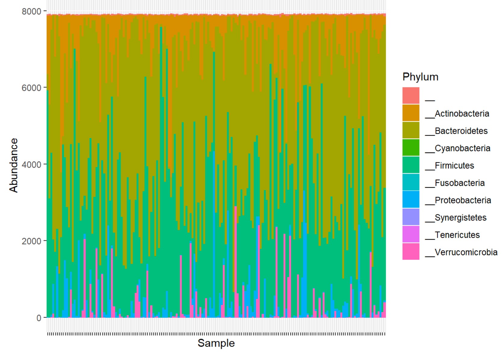
First of all, you need otu_table to draw a bar graph to see the abundance of each sample. Besides, since the total count of microbiome for each sample is different, if you want to proportion of OTU through a bar graph, you need to compute the relative frequency of the count. To convert the count value, you can do following.
rel_sum <- function(x) round((x/sum(x)))
rel_data = transform_sample_counts(data, rel_sum)
total = median(sample_sums(data))
standf <- function(x, t=total) round(t*(x/sum(x)))
stand_data <- transform_sample_counts(data, standf)
otu_table(data)[1:10, 1:5]
otu_table(rel_data)[1:10, 1:5]
You can draw a bar graph using ggplot2 package.
library(ggplot2)
plot_bar(stand_data, fill = "Phylum")+
  geom_bar(aes(color=Phylum, fill=Phylum), stat="identity", position = "stack")+
  theme(axis.text.x = element_blank())

Heatmap
If your data has the larger number of taxonomy, it would be better to filter your data in heatmap analysis. The following code is to extract the taxonomy whish has the larger counts than median by 10\%.
stand_data_abund <- filter_taxa(stand_data, function(x) sum(x>total*0.1)>0, TRUE)
stand_data_abund
When you create a heatmap, the result is following. ```{r, echo = F} plot_heatmap(stand_data_abund, method = “NMDS”, distance = “bray”)+theme(axis.text.x = element_blank())
<div class="row">
    <div class="col-sm mt-3 mt-md-0">


<figure

>
  <picture>
    <!-- Auto scaling with imagemagick -->
    <!--
      See https://www.debugbear.com/blog/responsive-images#w-descriptors-and-the-sizes-attribute and
      https://developer.mozilla.org/en-US/docs/Learn/HTML/Multimedia_and_embedding/Responsive_images for info on defining 'sizes' for responsive images
    -->

      <source
        class="responsive-img-srcset"
        srcset="/assets/img/img2_3-480.webp 480w,/assets/img/img2_3-800.webp 800w,/assets/img/img2_3-1400.webp 1400w,"

          sizes="95vw"

        type="image/webp"
      >

    <img
      src="/assets/img/img2_3.jpg"

        class="img-fluid rounded z-depth-1"


        width="100%"


        height="auto"


        title="example image"


        loading="eager"

      onerror="this.onerror=null; $('.responsive-img-srcset').remove();"
    >
  </picture>


</figure>

    </div>
</div>


### Alpha diversity

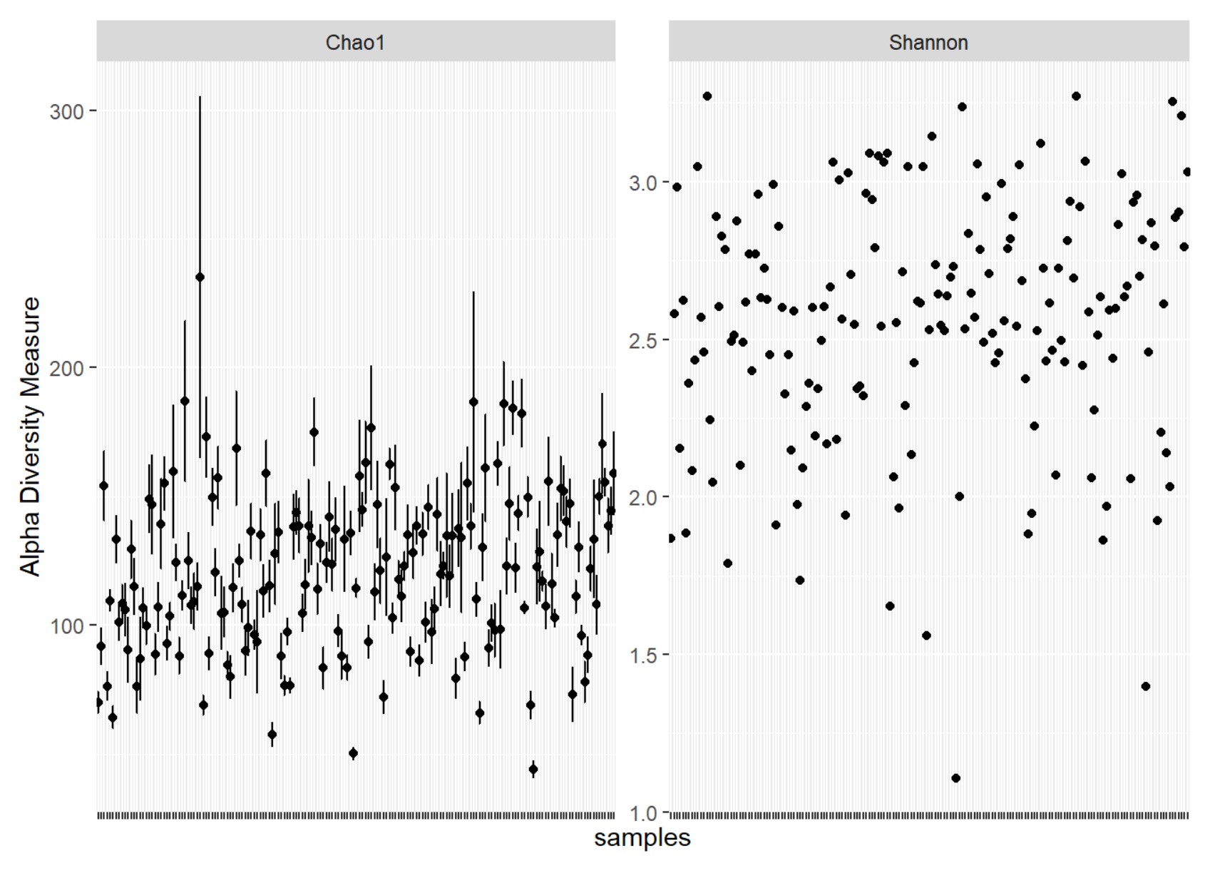
To compute alpha diversity, you can use *estimate_richness()* to obtain Chao1, Shannon, and Simpson.
```{r, results = 'markup'}
estimate_richness(data, measures = "Chao1") %>% head
estimate_richness(data, measures = "Shannon") %>% head
estimate_richness(data, measures = "Simpson") %>% head
plot_richness(data, measures = c("Chao1", "Shannon"))+theme(axis.text.x = element_blank())

Beta diversity
You can compute beta diversity by distance() function. ```{r, results = ‘markup’} distance(data, method = “unifrac”) %>% head distance(data, method = “wunifrac”) %>% head distance(data, method = “bray”) %>% head distance(data, method = “dpcoa”) %>% head
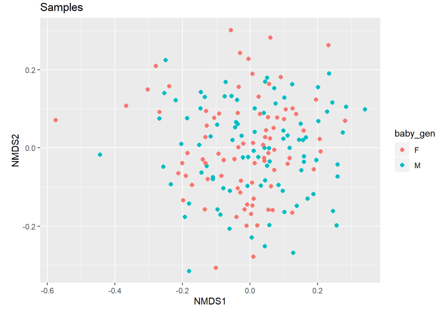
Since the beta diversity is a distance matrix, we need to reduce dimension using ordination. Ordinatiom includes methods *NMDS* and *PCoA*.
```{r, results = 'markup'}
data.ord1 <- ordinate(data, "NMDS", "bray")
data.ord2 <- ordinate(data, "NMDS", "wunifrac")
data.ord3 <- ordinate(data, "PCoA", "bray")
data.ord4 <- ordinate(data, "PCoA", "wunifrac")
plot_ordination(data, data.ord1, type="samples", title = "Samples", color = "baby_gen")+
  geom_point(size=2)
